Introduction to LCL

LCL is a framework for modelling, simulating and reasoning about dynamical systems.

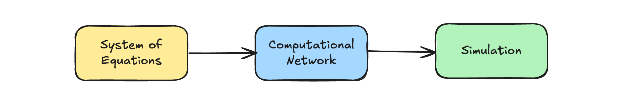
LCL has three main components: equations, networks and simulations.

Equations

A dynamical system is defined as a system of equations, which define the dynamics of the system. Examples of this would be a system of differential, or difference, equations.

Networks

Equations can then be translated into computational networks. Networks is a unified way of representing dynamical systems. We can use networks to both reason about dynamical systems as well as simulate them.

Simulations

Networks allow us to simulate to a given level of precision the approximation of the evolution of a dynamical system, given a particular set of initial conditions.

Features and advantages

Standard mathematical notation for defining systems

Systems can be defined in many, if not most, sensible ways, including as differential or difference systems, closed-forms, composed and dependent systems etc. All of which is defined in a standard, intuitive grammar, similar to common mathematical notation.

Supports a wide range of types of dynamical systems

LCL supports a range of dynamics and types of dynamical systems, including:

• Both deterministic and stochastic systems
• Linear and Non-linear
• Self-contained as well as composed systems
• Single and multi-dimensional dynamics

System definition is independent of underlying type

The definition and approximation steps of LCL are the same irrespective of the underlying calculus - whether deterministic or stochastic, real or complex. The difference in underlying calculi only matters at simulation stage, meaning the modelling and reasoning can be in the abstract.

Supports mixed underlying types

The network simulation step also allows a mixed of calculi to be instantiated at simulation time, meaning that each simulated variables calculi can be choosen independently.

Proof system for reasoning about models and simulations

LCL comes with a baked-in proof system for reasoning about dynamical systems based on the computational networks.

This enables several interesting applications:

• System Selection: finding systems to fit data sets either from scratch or from initial guess
• Reasoning about systems: proving properties about systems
• Algebraic Solving: mechanically finding closed-form solutions, or approximations, to systems

Supports distribution of computations

Because of the properties of computational networks, approximations and simulations can easily be distributed locally at operator level and remotely at sub-system level, meaning it can scale large systems and high fidelity simulations.

From equations to networks

When a system is defined in the equational notation (details here) it is translated into a computational network expressed in the network grammar (details here).

As mentioned above, this language provides a computational form of the system that allows us to reason about its construction, simulate its evolution over given calculi and construct computational equivalent networks with desired properties, like closed-form.

The translation from a system of equations to a single network follow a standard process:

1. Normalisation: Normalise each equation according to axioms of a differential real ring
2. Bounded Variables: Identify set of bounded variables for each equation
3. Solve Boundedness: Solve across system for bounding of variables
4. Isolate: Isolate each select bounded variable for each equation
5. Resolution: Resolve the operators on lhs and re-write to completely isolate the bounded variable
6. Translation: Construct computation networks for each resolved equation
7. Normalisation: Normalise each network by applying rewrite rules according to axiom of network category
8. Unification: Unify computational networks by through monoidal constructs and connecting identical inputs and outputs
9. Trace: Apply trace operators on the unified network by tracing outputs back to matching inputs

Simulating Networks

At approximation and simulation time we follow the following steps:

1. Set truncation length of approximation
2. Setup initial conditions, free variables and fixed function variables
3. Apply calculi specific rewrite rules to variable integrations, like Ito to Stratonovich translations
4. Compute approximation coefficients for expansion by running circuit on inputs
5. Either compute simulations at the same time or only compute appximation and run simulation after
6. Simulations are typically computed using Monte Carlo

Reasoning about Networks

TODO